<center> How to Plot Mathematical Functions in 10 Lines of Python === *Written by [Juan David Arias](https://github.com/juanArias8). Published 2021-06-08 on the [Monadical blog](https://monadical.com/blog.html).* </center> When I started studying Systems Engineering, I only had a basic knowledge of mathematics, and, to be honest, I saw it as a necessary evil: difficult and boring, but obligatory. My high school education had basically rewarded memorization more than reflection. There was no motivation to understand the foundations of mathematics or how it really worked--the idea was just to learn what problems a certain formula solved, memorize the right set of steps, and reproduce all of that for the exam. It was only when I started to learn about kinematics that I saw the magic of mathematics. Kinematics is often known as the “geometry of motion”: it’s the study of interactions between moving bodies over time. My professor of mechanical physics would stop in the middle of class and ask us to imagine these interactions and, to help us, he would program models of equations in [Wolfram Mathematica](https://www.wolfram.com/mathematica). Seeing a visual representation of mathematical functions like this made them come alive for me: I felt like I was understanding them properly for the first time. I decided to learn how to do data modelling for myself and began writing my own scripts. A few years later, I was invited by a friend to a talk on parametric curves. When the other attendees found out I had some experience in data modeling, they asked me if I could write a script for plotting parametric curves. I decided to give it a shot using Python, NumPy, SymPy, and Matplotlib. ## The script for plotting parametric curves Parametric curves are fascinating! In simple terms, a parametric curve can be understood as the trace left by the motion of a particle in space. To put things in a slightly more formal way, that trace is modeled by a function defined from an interval $I$ to various points in a space $E$. For the three-dimensional case, if $x$, $y$ and $z$ are given as functions of a variable $t$ in $I$, known as the parameter, we obtain the equations $x = f(t)$, $y = g(t)$ y $z = h(t)$. By evaluating each value of the parameter $t$ in each of these equations, we obtain a point $p(t) = (x(t), y(t), z(t))$ in space. If we perform the procedure for values of $t$ varying in an interval $I$, we obtain a parametric curve. After doing some research, trying some models by hand, and spending many hours working on the script, I came up with a solution. Here’s what that looks like: ```python import sympy as sp import numpy as np import matplotlib.pyplot as plt from mpl_toolkits.mplot3d import Axes3D t = sp.Symbol('t') function_x = sp.sympify('sin(t)') function_y = sp.sympify('cos(t)') function_z = sp.sympify('t**2') interval = np.arange(0, 100, 0.1) x_values = [function_x.subs(t, value) for value in interval] y_values = [function_y.subs(t, value) for value in interval] z_values = [function_z.subs(t, value) for value in interval] fig = plt.figure(figsize=(10, 10)) ax = plt.axes(projection='3d') ax.plot(x_values, y_values, z_values) plt.show() ``` 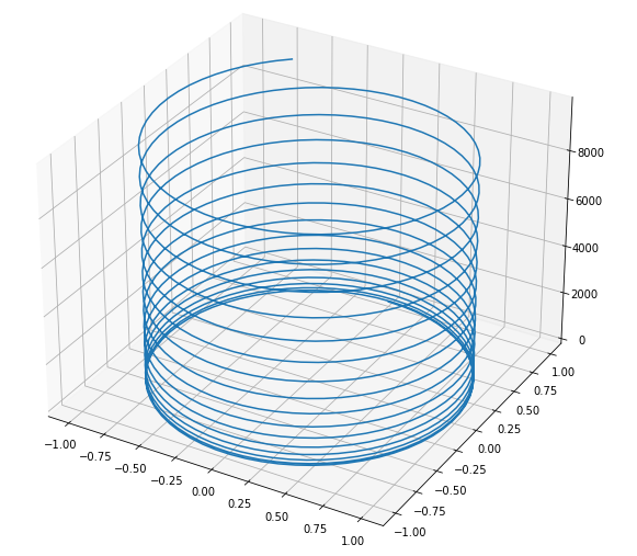This script allows us to generate graphs for parametric curves. Here’s the graph of the parametric helix $p(t) = (sin(t), cos(t), sqrt(t^3))$, for the interval $[0, 100)$. <center>  </center> ## How the script works The script makes use of the libraries SymPy, NumPy, and Matplotlib. **[SymPy](https://www.sympy.org/en/index.html)** is a Python library for symbolic mathematics. It aims to become a full-featured computer algebra system (CAS) while keeping the code as simple as possible in order to be comprehensible and easily extensible. SymPy is written entirely in Python. **[NumPy](https://numpy.org/doc/stable/user/whatisnumpy.html)** is the fundamental package for scientific computing in Python. It’s a Python library that provides a multidimensional array object, various derived objects (such as masked arrays and matrices), and an assortment of routines for fast operations on arrays, including mathematical, logical, shape manipulation, sorting, selecting, I/O, discrete Fourier transforms, basic linear algebra, basic statistical operations, and random simulation. **[Matplotlib](https://matplotlib.org/)** is a comprehensive library for creating static, animated, and interactive visualizations in Python. To use these libraries in our script, we must first install them on our computer by running the following instruction from the terminal: ```shell pip install numpy sympy matplotlib ``` We can now import them from our script: ```python import sympy as sp import numpy as np import matplotlib.pyplot as plt ``` The SymPy symbolic computations are done with symbols. SymPy variables are objects of the Symbols class. The `t = sp.Symbol('t')` assigns the symbol $t$ to the variable`t`, which from now on we can operate on as a mathematical variable. ```python t = sp.Symbol('t') print(t ** 2) >> > t ^ 2 ``` For this task, we need to work with compound expressions stored in a string. To make the conversion from a string to a mathematical expression understandable for SymPy, we make use of the `sympify` function. `sp.sympify(expression)` converts the parameter `expression` into a general mathematical expression. ```python function_z = sp.sympify('t^2') print(function_z + 2) >> > t ^ 2 + 2 ``` Now the variable `function_z` contains the mathematical expression $t^2 + 2$. The next step is to be able to evaluate the parameter $t$ inside the mathematical expression. The `subs` function of SymPy will allow us to evaluate an expression with a given value. We can use it in the following way: `expression.subs(t, value)`. ```python value = function_z.subs(t, 5) print(value) >> > 5 ^ 2 = 25 ``` Since we are talking about parametric functions, we are interested in evaluating the function on a sequence of real values within an interval (we use NumPy's `arange` function for this). The `np.arange(start, stop, step)` function creates a NumPy array with values in the half-open interval $[start, stop)$ with increments of `step`. ```python interval = np.arange(0, 10, 1) print(interval) >> > array([0, 1, 2, 3, 4, 5, 6, 7, 8, 9]) ``` Once the interval array is created, we need to iterate over the values of $t$ and evaluate each value inside the function. To do this, we’re going to use Python list comprehension and the `subs` function of SimPy. The `subs` function receives the symbol $t$ (that we have stored in the variable `t`) and the value of each item as parameters. ```python z_values = [function_z.subs(t, value) for value in interval] print(z_values) >> > [0, 1, 4, 9, 16, 25, 36, 49, 64, 81] ``` We repeat the procedure for the values of `x_values` and `y_values` and so obtain the arrays with the values to plot. Finally, with the help of Matplotlib, we show the graph corresponding to the parametric curve. 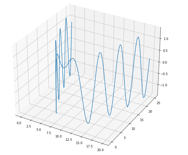In the three-dimensional case, we use the following statement to indicate to Matplotlib that we want to make a three-dimensional graph: ```python ax = plt.axes(projection='3d') ``` We can replace the functions and the interval and obtain new and infinite curves. Let's try it again with different values. ```python function_x = sp.sympify('2*t + 10') function_y = sp.sympify('t**2') function_z = sp.sympify('sin(t**2) + cos(t**2)') interval = np.arange(-5, 5, 0.05) ``` <center>  </center> ## Playing around During my research, I came across a variety of shapes that could be created using parametric curves. I found that some combinations could generate curves with a unique symmetry and beauty. If you want to play around with the script yourself, you can open [this link](https://trinket.io/python3/791f8b4319?runOption=run) and replace the values for `function_x`, `function_y`, `function_z`, and `interval`. 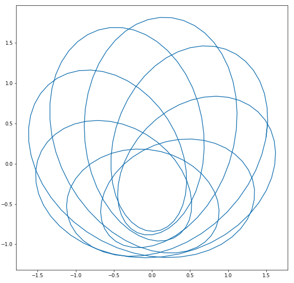<iframe src="https://trinket.io/embed/python3/c6abaec211?runOption=run&start=result" width="100%" height="356" frameborder="0" marginwidth="0" marginheight="0" allowfullscreen></iframe> ## Modifying the script for 2D parametric curves With some modifications, the script can also be used to plot two-dimensional parametric curves. Here’s the two-dimensional plot generated by evaluating $x = t - 1.6*cos(24*t)$ and $y = t - 1.6*sin(25*t)$ on an interval $I = [1.5, 20.5]$. 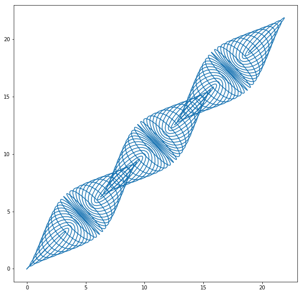<center>  </center> The parametric curve shown above can be modeled in Python with the following script: ```python import sympy as sp import numpy as np import matplotlib.pyplot as plt t = sp.Symbol('t') function_x = sp.sympify('t - 1.6*cos(24*t)') function_y = sp.sympify('t - 1.6*sin(25*t)') interval = np.arange(1.5, 20.5, 0.01) x_values = [function_x.subs(t, value) for value in interval] y_values = [function_y.subs(t, value) for value in interval] plt.figure(figsize=(10, 10)) plt.plot(x_values, y_values) plt.show() ``` Let's test it with other functions and a new interval: ```python function_x = sp.sympify('4*sin(5*t)') function_y = sp.sympify('5*cos(3*t)') interval = np.arange(0, 6.5, 0.001) ``` <center>  </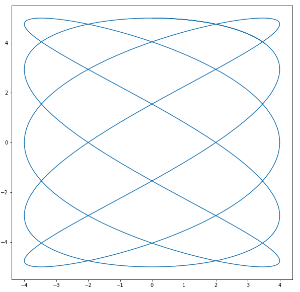center> And one more time... ```python function_x = sp.sympify('cos(16*t) + (cos(6*t) / 2) + (sin(10*t) / 3)') function_y = sp.sympify('sin(16*t) + (sin(6*t) / 2) + (cos(10*t) / 3)') interval = np.arange(0, 3.16, 0.01) ``` <center>  </center> Amazing! If you want some more examples of interesting curves, check out these links: * https://www.quora.com/What-are-the-most-interesting-equation-plots * https://co.pinterest.com/pin/115123334204984317 * https://co.pinterest.com/fredsolidstate/parametric/ ## Building a mathematical function plotter Once I finished the script for modelling parametric curves, I realized that with very few lines of code I could generate a plotter for mathematical functions in both two and three dimensions! Here’s the script for generating plots of mathematical functions in two and three dimensions within the interval $[a, b]$. The console will ask the user for both the function and the values a and b of the interval. ```python import sympy as sp import numpy as np import matplotlib.pyplot as plt from mpl_toolkits.mplot3d import Axes3D symbol_x = sp.Symbol('x') symbol_y = sp.Symbol('y') def get_vector(a, b): return np.arange(a, b + 1, 0.1) def plot_2d_function(function, a, b): # Create the sympy function f(x) f_x = sp.sympify(function) # Create domain and image domain_x = get_vector(a, b) image = [f_x.subs(symbol_x, value) for value in domain_x] # Plot the 2D function graph fig = plt.figure(figsize=(10, 10)) plt.plot(domain_x, image) plt.show() def plot_3d_function(function, a, b): # Create sympy function f(x, y) f_xy = sp.lambdify((symbol_x, symbol_y), sp.sympify(function)) # Create domains and image domain_x = get_vector(a, b) domain_y = get_vector(a, b) domain_x, domain_y = np.meshgrid(domain_x, domain_y) image = f_xy(domain_x, domain_y) # Plot the 3D function graph fig = plt.figure(figsize=(10, 10)) ax = plt.axes(projection='3d') ax.plot_surface(domain_x, domain_y, image, rstride=1, cstride=1, cmap='viridis') plt.show() function = input('>> Enter the function: ') a_value = float(input('>> Enter the [a, ] value: ')) b_value = float(input('>> Enter the [, b] value: ')) if "x" and not "y" in function: plot_2d_function(function, a_value, b_value) elif "x" and "y" in function: plot_3d_function(function, a_value, b_value) else: print("You must enter a function in terms of x and/or y") ``` You can test this script for yourself [here](https://trinket.io/python3/23f8ad681c?runOption=run): run the script and enter your own configuration. <iframe src="https://trinket.io/embed/python3/181bde2cb7?runOption=run&start=result" width="100%" height="356" frameborder="0" marginwidth="0" marginheight="0" allowfullscreen></iframe> *Two dimensional function plot* <iframe src="https://trinket.io/embed/python3/fa70d45632?runOption=run&start=result" width="100%" height="356" frameborder="0" marginwidth="0" marginheight="0" allowfullscreen></iframe> *Three dimensional function plot* In my next few posts, I’ll be explaining how to work with fast API, React, Unity, Vuforia and augmented reality, to build an interactive system of visualizations of graphs of mathematical functions. <center>  </center> <center> <img src="https://monadical.com/static/logo-black.png" style="height: 80px"/><br/> Monadical.com | Full-Stack Consultancy *We build software that outlasts us* </center>